Scott Hosking
For this notebook to work you will need to install:
import baspy as bp
import matplotlib.pyplot as plt
import cartopy.crs as ccrs
import xarray as xr

%matplotlib inline
Using BASpy
Define the CMIP5 data we want to work with
catlg = bp.catalogue(dataset='cmip5', Experiment='historical',
                         Frequency='mon', Var='tas',
                         Model='HadGEM2-ES')
catlg.drop(columns=['Path','DataFiles'])
Updating cached catalogue...
catalogue memory usage (MB): 28.786099
>> Current cached values (can be extended by specifying additional values or by setting read_everything=True) <<
{'Experiment': ['piControl', 'rcp85', 'historical', 'rcp26', 'rcp45'], 'Frequency': ['mon']}
| Centre | Model | Experiment | Frequency | SubModel | CMOR | RunID | Version | Var | StartDate | EndDate | dataset | |
|---|---|---|---|---|---|---|---|---|---|---|---|---|
| 489465 | MOHC | HadGEM2-ES | historical | mon | atmos | Amon | r2i1p1 | v20110418 | tas | 185912 | 200512 | cmip5 |
| 489511 | MOHC | HadGEM2-ES | historical | mon | atmos | Amon | r4i1p1 | v20110418 | tas | 185912 | 200511 | cmip5 |
| 489557 | MOHC | HadGEM2-ES | historical | mon | atmos | Amon | r3i1p1 | v20110418 | tas | 185912 | 200512 | cmip5 |
| 489605 | MOHC | HadGEM2-ES | historical | mon | atmos | Amon | r1i1p1 | v20120928 | tas | 185912 | 200511 | cmip5 |
Select one model run (one row)
row = catlg.iloc[3]
row
Centre                                                     MOHC
Model                                                HadGEM2-ES
Experiment                                           historical
Frequency                                                   mon
SubModel                                                  atmos
CMOR                                                       Amon
RunID                                                    r1i1p1
Version                                               v20120928
Var                                                         tas
StartDate                                                185912
EndDate                                                  200511
Path          /MOHC/HadGEM2-ES/historical/mon/atmos/Amon/r1i...
DataFiles     tas_Amon_HadGEM2-ES_historical_r1i1p1_185912-1...
dataset                                                   cmip5
Name: 489605, dtype: object
Using Xarray
At this point (if the data is stored on the system we are on) we can read in multiple files as a Dataset using: ds = bp.open_dataset(row)
However, assuming you do not have access to the CMIP5 or CMIP6 data archive, you can download and get going with some CMIP6 sample data by running this line:
ds = bp.eg_Dataset()
ds
<xarray.Dataset>
Dimensions:    (bnds: 2, lat: 180, lon: 288, time: 420)
Coordinates:
  * bnds       (bnds) float64 1.0 2.0
    height     float64 ...
  * lat        (lat) float64 -89.5 -88.5 -87.5 -86.5 -85.5 -84.5 -83.5 -82.5 ...
  * lon        (lon) float64 0.625 1.875 3.125 4.375 5.625 6.875 8.125 9.375 ...
  * time       (time) datetime64[ns] 1980-01-16T12:00:00 1980-02-15T12:00:00 ...
Data variables:
    lat_bnds   (lat, bnds) float64 ...
    lon_bnds   (lon, bnds) float64 ...
    tas        (time, lat, lon) float32 ...
    time_bnds  (time, bnds) datetime64[ns] ...
Attributes:
    title:                 NOAA GFDL GFDL-AM4 model output prepared for CMIP6...
    history:               File was processed by fremetar (GFDL analog of CMO...
    table_id:              Amon
    contact:               gfdl.climate.model.info@noaa.gov
    comment:               <null ref>
    tracking_id:           hdl:21.14100/3b95ceac-9bd6-42c9-a130-130fc1ba108c
    further_info_url:      https://furtherinfo.es-doc.org/CMIP6.NOAA-GFDL.GFD...
    branch_time_in_child:  0.0
    branch_method:         no parent
    creation_date:         2018-08-07T17:02:18Z
    Conventions:           CF-1.7 CMIP-6.0 UGRID-1.0
    sub_experiment:        none
    frequency:             monC
    forcing_index:         1
    physics_index:         1
    initialization_index:  1
    realization_index:     1
    parent_variant_label:  no parent
    parent_experiment_id:  no parent
    data_specs_version:    01.00.27
    experiment_id:         amip
    experiment:            AMIP
    activity_id:           CMIP
    source_id:             GFDL-AM4
    source_type:           AGCM
    institution_id:        NOAA-GFDL
    institution:           National Oceanic and Atmospheric Administration, G...
    variable_id:           tas
    variant_info:          N/A
    mip_era:               CMIP6
    source:                "GFDL-AM4 (2017): aerosol: interactive;atmos: GFDL...
    parent_activity_id:    no parent
    parent_mip_era:        no parent
    parent_source_id:      no parent
    parent_time_units:     no parent
    sub_experiment_id:     none
    grid:                  atmos data regridded from Cubed-sphere (c96) to 18...
    variant_label:         r1i1p1f1
    grid_label:            gr1
    license:               CMIP6 model data produced by NOAA-GFDL is licensed...
    nominal_resolution:    100 km
    product:               model-output
    realm:                 atmos
    references:            see further_info_url attribute
# read a DataArray (e.g., a single variable) from the Dataset
da = ds.tas
da
<xarray.DataArray 'tas' (time: 420, lat: 180, lon: 288)>
[21772800 values with dtype=float32]
Coordinates:
    height   float64 ...
  * lat      (lat) float64 -89.5 -88.5 -87.5 -86.5 -85.5 -84.5 -83.5 -82.5 ...
  * lon      (lon) float64 0.625 1.875 3.125 4.375 5.625 6.875 8.125 9.375 ...
  * time     (time) datetime64[ns] 1980-01-16T12:00:00 1980-02-15T12:00:00 ...
Attributes:
    long_name:      Near-Surface Air Temperature
    units:          K
    cell_methods:   area: time: mean
    cell_measures:  area: areacella
    standard_name:  air_temperature
    interp_method:  conserve_order2
    original_name:  tas
Plotting
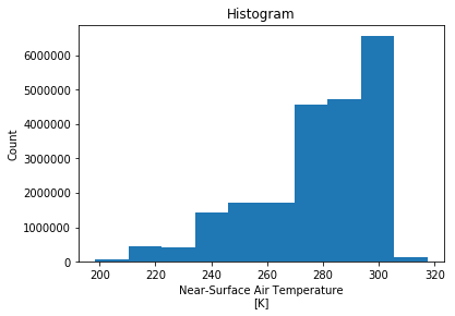
da.plot()
(array([  69415.,  442264.,  428669., 1430675., 1719399., 1709979.,
        4552300., 4731607., 6553416.,  135076.]),
 array([198.42273, 210.32277, 222.22281, 234.12283, 246.02287, 257.9229 ,
        269.82294, 281.723  , 293.62302, 305.52307, 317.4231 ],
       dtype=float32),
 <a list of 10 Patch objects>)
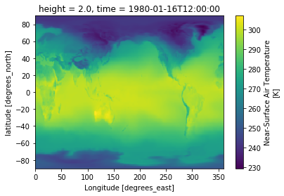
Plot map for first time index
da.isel(time=0).plot()
<matplotlib.collections.QuadMesh at 0x3292b76a0>
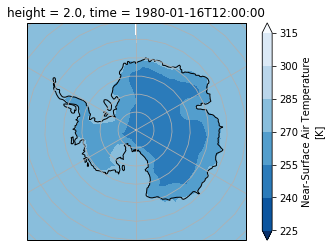
Plot using a polarstereo map projection
crs = ccrs.SouthPolarStereo(central_longitude=0.0)
ax = plt.subplot(projection=crs)
ax.set_extent([-180,180,-90,-60], ccrs.PlateCarree() )
ax.gridlines(ylocs=range(-90,-30,5))
da.isel(time=0).plot.contourf(ax=ax, transform=ccrs.PlateCarree(),
                                  cmap=plt.cm.Blues_r,
                                  extend='both')
ax.coastlines('110m', color='k')
<cartopy.mpl.feature_artist.FeatureArtist at 0x32af969e8>